Model training

# Imports 
import cv2
import numpy as np
import pandas as pd
import matplotlib.pyplot as plt
from mpl_toolkits.mplot3d import Axes3D
import pickle
import pandas as pd
from sklearn.preprocessing import LabelEncoder 
from sklearn import svm

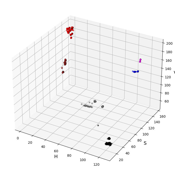
Before training, we will first analyze the dataset. This is a 3D HSV-color space in which every point represents a color band of a resistor in the image dataset.

# Load data
df = pd.read_csv("../data/color_data.csv")
c=df['Class'].map({'x':'gray','r':'red','z':'brown','k':'black','b':'blue','v':'magenta','g':'green'})

# Plot
fig = plt.figure(figsize=(12, 9))
ax = fig.add_subplot(111, projection='3d')
ax.scatter(df.H, df.S, df.V, c=c, alpha=.6, edgecolor='k', lw=0.3)
ax.set_xlabel('H', fontsize=14)
ax.set_ylabel('S', fontsize=14)
ax.set_zlabel('V', fontsize=14)
plt.show()

Next, we load the data which contains three feature columns (H, S, and V) and one class column. The labels are encoded before passing to the classifier.

# Load data
df = pd.read_csv("../data/color_data.csv")

# Encode categorical labels
labelencoder= LabelEncoder() 
df['Class'] = labelencoder.fit_transform(df['Class'])

# Fill missing values
df.fillna(0, inplace=True)

# Train
clf = svm.SVC()
clf.fit(df[['H', 'S', 'V']].values, df['Class'].values)

SVC()

In a Jupyter environment, please rerun this cell to show the HTML representation or trust the notebook.
On GitHub, the HTML representation is unable to render, please try loading this page with nbviewer.org.

Lastly, the model will be saved for further use.

# Save model
filename = '../data/model.sav'
pickle.dump(clf, open(filename, 'wb'))